ERM and DFA using Active Structure
Jim Brander
Interactive Engineering
Email: jim.brander@pacific.net.au
Sam Manoff
Tupai Business Systems
Email: smanoff@tupaisystems.co.il
Abstract
Introduction
This paper addresses the following areas:
| Correlation/dependency: The storing of correlations and dependencies | |
| Integration: Methodology for integrating correlated risk distributions into models | |
| Dependency/causal models: The modeling of risk defined by presumed causes |
Lying behind these areas of interest is an increasing interconnectedness and dynamicity of the risk environment – conditions which current analytic tools do not well support. Tools now implement one of several techniques - the ‘natural order’ of calculation of spreadsheets (which must be known in advance of any calculation), directed dataflow or specific programming using a single point of control. None of these techniques is appropriate for interdependent risks, where the nature of the interaction is dynamic.
We will attempt to show that an undirected structure with distributed control and comparatively complex messaging, and with the abilities to store experiential knowledge within its structure and to modify its own structure, addresses the areas mentioned above. The resulting model looks very much like current analytic models – it is just that the underlying process that propagates information is very different.
Restriction on Information Transmission leads to a Disconnect
A model is intended to assist in analysing a complex situation. The representation of enterprise risk, involving as it does probability and the connections among different risks, is a complex problem, modeled only with difficulty. Unfortunately, much of the current modeling effort is disconnected from the actual problem, and instead turns on artifacts of the analytic modeling process, as the following diagram seeks to illustrate.
Figure 1 (after [5])
Deciding whether the association between two risks is Gaussian or Gumbelian would seem to be far from the actual problem. Large events are rare, so a few more events can quickly invalidate any a priori modeling decision. The other aspect with risk events in extremis is that the extreme events are likely to involve size or resource thresholds and thus processes that simply do not apply in less extreme events – a large, critically situated, earthquake could destroy stockmarkets around the world, whereas there is no correlation with a small tremor. That is, large risks are much more likely to be interconnected because the large-scale processes they unleash will overlap. The current methods of closed form analysis handle interdependence poorly. This may be one reason for the popularity of DFA using simulation, as the cyclic nature of simulation appears to allow interdependence to be handled with minimal effort. This is somewhat of an illusion, particularly when a risk is spiked as part of a simulation.
We begin by examining whether the statistical methods of current risk modelling methods are appropriate or necessary
When the only object in an analytic model that can be propagated is a number or a group of numbers, description of the risk must be turned into, at most, a few numbers that act as parameters – a type of distribution, a variance, possibly a skew, a correlation, a copula. This restriction, whether for insurance or finance or engineering, is artificial – it declares a clarity of parameter and an initial precision that does not exist in the messy world we are attempting to model. The actuarial literature has many examples where the author points out that the distributions involved are far from Gaussian, and then proceeds to use the method anyway, for want of something better.
Beginning a calculation with a number asserts that there is a seed that can be known precisely. This is valid for a payroll application, where the rate per hour is known for a particular employee and operations on this seed will yield a valid result – it is not valid where a calculation must start with multiple risks which are interdependent and known only by their probability distributions, or where the end result is non-monotonic – an example is interest rates, where very low and very high values both lead to asset inflation. Some dependencies, such as an earthquake causing fires, are directional, allowing a simple directed approach. Whether in their language or in their mental models, humans do not rely on precise numbers to begin their processing, but rather on influences and associations, although the end result of the mental activity can still have astounding precision. If we broaden what we can propagate in our analytic models to allow for the propagation of numeric ranges and the storage of distributions and stochastic associations, then many of the limitations of current analytic modeling techniques using singular values disappear.
Numbers in analytic models are typically represented by values in memory that can be loaded into a register at the behest of a procedure, and there manipulated. Let us instead use a network object to represent a number – something with existence, attributes and the ability to be linked. As a very brief introduction to knowledge networks, we offer the equation shown in Figure 2.
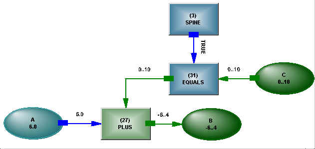
Figure 2 – A + B = C
The structure is made up of variables, operators (PLUS etc.) and links. As shown, the variable A has a singular value and C has a range, and these two values have been combined at the PLUS operator to produce a value which is propagated to B – the direction of information flow was dynamically determined [2]. The SPINE operator, in the top center of the diagram, functions as an AND, connecting and controlling all the statements in the model, allowing the model to become a controllable submodel in a larger model if desired. A True logical state from the SPINE has enabled the EQUALS operator to propagate the value from C. As states and values of the variables come and go, the direction of information transmission in the structure may change, reflecting the current state (direction of propagation is part of that state). The undirected nature of the structure means that it is initially uncommitted as to purpose – useful when dealing with situations such as interdependent risk, where the influence can come from any direction. Operators only perform calculations when the logical states on their connections change, so that the network micro-schedules its activity, and no external control algorithm is required – a desirable feature as complexity grows. To elaborate a little more, we may have the statement
IF A + B = C THEN D + E = F
The numeric elements embedded in the logical statement look like the a-b-c structure we have already encountered. In the interests of generality, it would seem reasonable to use identical structure in both places in the statement. If we implement the logical part of the statement as sentential logic, we have the arrangement shown in Figure 3.
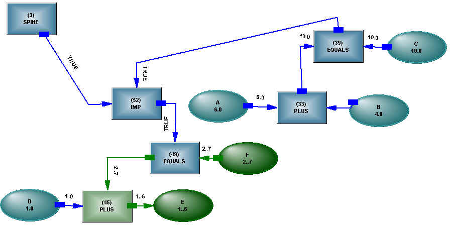
Figure 3 – IF A + B = C THEN D + E = F
The IF...THEN... is implemented as a logical implication, and the logical operator also responds to changes in logical states on its connections. The example shows structures as components in a larger structure, and we have retained all the possible inferences - modus tollens, for example. This allows the system to reason about the cause when an effect is not as expected.
Without going into details, there are structural analogs of the usual programming machinery - FOR and WHILE loops (see [3]), fetch and store operations, sigma and other analytic operators used in actuarial models, string, list and object handling – all involving identifiable states in structure.
The foregoing may give the impression of merely a graphical representation of textual statements, but that would be a false impression. As relations become dense and complex, graphical representations except at a high level of abstraction are much harder to comprehend than textual representations– the many-variabled relationship between earthquake magnitude and damage shown in [1], for example. Instead, the text of an analytic statement is converted into a structure, a structure which stores its current state inside itself and propagates states and values through its connections, and which interacts with the structure produced by other statements. What distinguishes this structure from a graph is its ability to alter its connections – to form what appears to be a new graph while the structure (the totality of states and connections) remains invariant. This may seem an unusual occurrence, so
X = SUM(List)
will serve as a common example. Some calculation is involved in determining the list, and we don’t yet know if we are working out the value of X or some member of the list, based on X and other values we find, and we need to recover our original state if the value for the list is lost. The underlying paradigm is of an active, undirected, extensible and self-modifying structure, rather than statements generating a sequence of instructions or a graph that is "understood" and operated on by an external algorithm. The knowledge network structure can appear very similar to the dataflow paradigm, where inputs flow to an operator, which then produces an output, which flows to another operator as an input, and so on until calculation is complete. The dataflow paradigm, however, assumes that the flow path of the information can be predetermined, directions remain fixed and the declared topology is invariant.
More Complex Messages
To use numeric ranges effectively, we actually need to go one step back in how our models work. If we have a number that is calculated in a model, exactly when can we access that number. Obviously, when the calculation is finished – but the calculation may be waiting on another calculation, and so on. And we may be using the statement as a statement rather than procedurally – that is, if we have
A = B + C
we may be working out C based on values for A and B. At this point, someone may object that "But I only want to work out A, not anything else". If we wish to work out interdependent risks, and the interdependence needs to be dynamically determined, then we should allow the model to determine the situation, not hope that we can program it in advance. If we associate a state with the number, the state tells us whether the number is valid. If we are to use a state, it can’t be a Boolean state – we may not yet have found the number but are still looking for it, or perhaps we failed to find it, or we may have encountered an error in the process. We already have True and False when handling logical variables, so let us use False as the state to indicate that we have a numeric range rather than a single value. The numeric range is also an object (itself comprised of objects), so it can be
An integer range 1..10
A real range 2.35<->7.9
The range does not have to be contiguous, so -3..5, 7..21, 43..1000000 is acceptable. These range objects are dynamically constructed and propagated, so the limits of the range do not have to be known beforehand. The Modus Tollens inference we mentioned has value in a statement like IF A < B THEN C > D, where influences flow in any direction rather than a test causes an action.
By allowing numeric ranges on variables to interact and cut each other in the manner of Constraint Reasoning – that is, information can flow back and forth on a connection - a continually reducing solution space is obtained. This reducing space, driven by many interacting influences, permits the solution of interdependent risk in closed form analysis.
Distributions and Means of Correlation
But ranges aren’t enough – for problems involving uncertainty, we need to represent probability over a range – a distribution. A discrete distribution is clunky if we can only use numbers to represent the different bins – the increment between the bins needs to be a preset constant. Now that ranges are available to be used for the bin limits, the ranges can be adaptive, with the bins wide where hits (occurrences) are few, narrow for precision where hits are many, and nonexistent where there are no hits (that is, the range for each bin is contiguous, but the ranges need not be contiguous). Figure 4 shows a simple example of a distribution (the value on the Y axis is number of occurrences within the range at its foot, making it an occurrence distribution rather than a probability distribution, but it is easily converted, based on the current range):
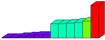
Figure 4 – Probability Distribution
With the real distribution represented with reasonable fidelity in the model, reliance on Gaussian and other analytically manageable distributions can be eased. The machinery in the network to support the distribution of the variable XX looks like
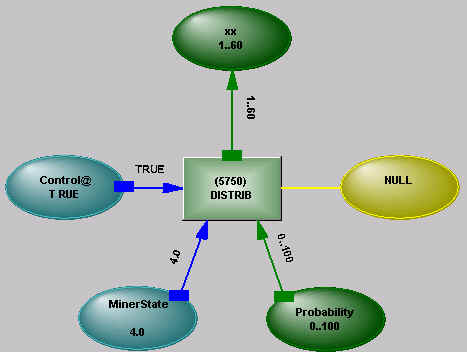
Figure 5 - DISTRIB Operator
Depending on a control state, the DISTRIB operator either "learns" from values arriving at its variable (storing occurrences in different ranges), or makes available a distribution from the values stored within it – the operator responds to logical states being communicated to it and its connections allow information to flow in any direction. The range of the distribution can be controlled by constraints acting on its variable – if X has a range of 1..50 and a distribution on that range, then introducing a constraint such as X < 20 will cut the range and truncate the distribution (it will temporarily put occurrences outside the constrained range at zero).
Where there is complex interrelated information, separate distributions alone do not represent the information adequately. A RELATION operator is used to connect the variables and control the distributions. Figure 5 is a simple example of a two dimensional relation (a maximum of ten dimensions is permissible).
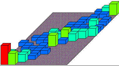
Figure 6 – Building Type vs Earthquake Damage - see [1]
The detailed map that the Relation provides between occurrences in distributions in different dimensions allows the detection of correlations that are smeared away by less detailed representations. The machinery to support the RELATION operator looks like
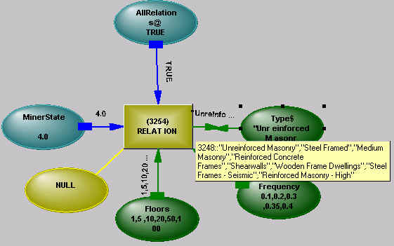
Figure 7 - Relation Operator
A change of distribution at one variable causes a change in distribution at other related variables. In the extreme case, if one variable is set to a singular value, then the other distributions are created by combining the values in the other dimensions corresponding to that value, as Figure 8 shows.
Figure 8 – Singular Value for Relation
Here, setting X1 to 4 has produced a distribution for Y1 based on the available data - real data can be rather sparse, so the contents of the distributions and relations may have been tidied up beforehand. The point is that real data has been used for the transformation between dimensions, rather than analytic approximations. The RELATION is undirected, so asserting a singular value or decreased range for Y1 would create a new distribution for X1. More commonly, the range of one variable would reduce due to some constraint. This would change the distributions of the other variables, which may cause a constraint in another dimension (or group of dimensions) to become active, further reducing distributions related to it. In this way, interdependent risks are handled naturally in closed form analysis, in a manner not dissimilar to the solving of simultaneous equations, except here they are a mixture of simultaneous stochastic and analytic relations.
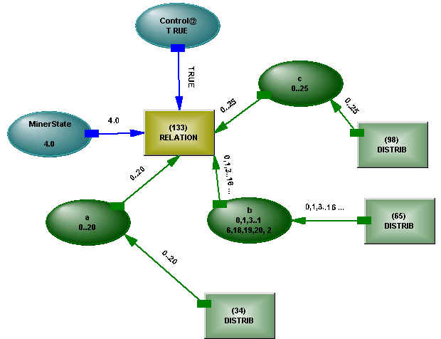
Figure 9 - Stochastic Analog
The structure shown in Figure 8 provides a stochastic analog of the structure shown in Figure 2 for the analytic statement A + B = C. A change in range on any of the variables will affect the distributions of the other variables. The Control connection on the relation mirrors the logical connection on the EQUALS operator, allowing the operator to be turned on and off.
Other operators in the network, triggered by changes of state, can extract any desired statistical measures from the dynamic states of the distribution and relation operators. RANDOM operators, when operating on variables with distributions, will pluck out a value based on the current distribution for that variable and set the variable to that value. Immediately, any variables linked through relation operators will have their distributions reduced, and RANDOM operators acting on them will find a value in their new distributions.
Using relation operators directly between seemingly interdependent risks may not be the most appropriate way to connect them if we have some idea of causality. An example is residential fire claims and motor vehicle claims. If there is asset deflation, we can expect both types to rise due to fraudulent claims. However, if there is a period of abnormally low precipitation, we can expect fire claims to rise because of wildfires and motor vehicle claims to fall because of dry roads. The example also undermines the static view of risk that is usually taken on the liability side – drought may require several years to set the scene for wildfires. If we can find causes for change, and these causes flow to several risks, our results will be much more precise if we manipulate causal variables than if we smear several causes by linking directly between risks. We have already mentioned that distributions and relations have a Learn state, where data is fed into them. There can be an arbitrary amount of analytic structure between the input data and the distributions/relations, allowing causal structure to be hypothesized and validated during the Learn phase. The ability to freely mix analytic and stochastic structure allows for steadily increasing precision, the analytic structure slowly encroaching on the stochastic structure as more is understood. Equally, analytic structure can extend the reach of stochastic structure where there is no history. An example of a complex risk, described by a combination of analytic and stochastic structure and requiring continual update of the structure, is given in [1].
We have shown how stochastic information may be embedded in a model to represent interrelated risks, but the conference call specifically describes the problem of combining stochastic and hypothetical risks. This may occur in several ways:
and the coupling of these two cases in any combination.
Take the example shown, where stochastic information is used inside the rectangle A, a mixture of stochastic and hypothetical is used inside rectangles B and C, and only hypothetical risk is used inside rectangle D, where any historical data may be nonexistent or out of date (in other words, one large disaster has rendered prior experience irrelevant).
Figure 10 - Hypothetical and Historical Risk
The easiest way to handle this is to augment the historical risk or create new risk distributions by using analytic structure to generate new data points in the model, the distribution and relation operators continuing in the Learn state until sufficient detail has been generated for the hypothetical component of risk. If the hypothetical risk needs to respond to current conditions in the model, then a different, dynamically switching, approach needs to be used. As an illustration, Figure 10 shows stochastic and analytic probability elements being combined dynamically.
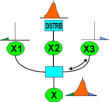
Figure 11 - Dynamically Combining Risk
Activation at any of the components X1 etc. leads to activation of the distribution operator connected to the variable X, and vice versa. This diagram illustrates the undirected nature of the structure, influences flowing at a low level wherever they will. With a little more modeling effort, the crossover points between the stochastic and calculated components of the risk can also be dynamically determined.
A Dynamic Environment needs Knowledge
Actuarial analysis has for a long time relied on the relative stability of the data being analyzed. Models could be built with little concern for maintainability – there certainly would be no major change in their structure over their life. Recent events have demonstrated how rapidly new risks may appear, and even if their primary effects can be avoided by rewriting policies, their secondary effects cannot. It is now desirable to have models which can be quickly adapted to changing circumstances (it always was, we needed a shock to remind us). If we look at the programmatic approach to building models, we see the cognitive scaffolding (the modeler) being used to build the model, and then being removed from it before the model is put into operation. The modeler needs to have anticipated any change in topology in the model and provided instructions to handle these. New risks, or the realization of some interconnectedness among existing risks, will often invalidate the topology the modeler has constructed, resulting in slow adaptation to change (or resistance to change because of the large intellectual investment in the existing model, and the sensitivity of programmatic models to topological change).
An alternative approach is to use the undirected knowledge network structures we have described. Each element in the structure determines direction of flow dynamically, so changes in topology can be made without requiring overall dataflow to be recast in the modeler’s head. The interconnecting logic is basically sentential (extended to handle errors and unknowables), allowing the model to reason about what is happening (and reducing the distance between our understanding of the model’s operation and our thinking about what needs to be done). That is, not so much of the cognitive support structure is removed when the model is placed in operation. The undirectedness of the structure results in the property of extensibility – structures can be combined easily because the phasing of the operation is implicit in the elements of the component structures.
As we have shown, embedding activity in the structure makes it simple to combine analytic and stochastic knowledge, and allow them to interoperate without the crudity of curve-fitting. In reasonably complex applications such as DFA, the analysis times for knowledge structures are comparable with programmatic methods – flow direction in the network is determined dynamically, but will not change unless there is a change to the input of the analysis that determined it.
Learning from Simulation
doing 100,000 simulations ... but I don’t think it actually helps you answer some of the fundamental questions. [4]
Simulation, correctly done, should help you answer some of the fundamental questions. If we take the example of a pilot on a flight simulator, it is not desired to have a report which shows that the pilot crashes 10% of the time – instead, it is desired that the pilot change his/her behavior in real situations as a result of simulated exposure to difficult conditions. Similarly in insurance, simulation is not about giving graphs to management, it is about learning from the experience. It is also not about
trying to precisely quantify some losses in ten years time, it is working out what management response might be compared to what it should be as certain patterns begin to appear in the market.If people resolutely refuse to look at what the DFA simulations are telling them (and with good reason - many of the simulations may be nonsensical due to the crudity of the embedded strategy), then perhaps it is appropriate to introduce some machine learning into the simulation. Machine learning may sound esoteric, but it is easily done by using the same distribution/relation operators as hold the stochastic information for the simulations in the first place, and allowing the results of simulation runs to modify their contents, and their contents to be used to control the simulation runs, so the system "learns" what is required to increase profits and avoid ruin. The obvious difficulty with this approach is that management sees from the simulations that ruin is unlikely, without understanding what the simulation model is doing to avoid it.
A reaction to meaningless simulation has resulted in increased interest in closed form analysis such as RAROC. The conceptual difficulty with a one period analysis like RAROC is that the insurance company followed a particular trajectory to reach the start of the period, and that trajectory is embedded in the mental models of management, thus controlling their strategic viewpoint – it is a simulation over a number of periods, with only the last period evaluated explicitly, the prior periods being implicit in the strategy. A company that had reached the same point by following a different trajectory would probably make very different decisions for the same future period. The strategy that is initially embedded in the simulation should represent current thinking (conditioned by its trajectory), and the simulation can then show how that strategy would operate as the simulation moves from now into the future (and the strategy changes in response to a changing situation). The actual dates into the future are irrelevant, except to act as a brake on how quickly adverse conditions can materialize (and how quickly the mental models of management will change in response to the effects of those adverse conditions).
Conclusion
Knowledge structures can remove many of the obstacles to representation of complex risks. Their undirected nature and active consistency maintenance allows for rapid, controlled, changes to a complex model in the face of changing circumstances. Their intrinsic property of self-modification introduces a dynamic structure, an ability to represent complex strategy and a self-learning ability to DFA for the first time.
References