A current method of risk analysis for a project is to develop a project plan using the Critical Path Method (CPM), then determine where there is risk of failure. Risk is often analysed by splitting it into its component effects on Duration, Cost and Outcome. This form of external risk analysis, no matter how detailed, becomes an addendum to the plan. The CPM plan itself may be quite unrealistic as a model of the project, particularly where development or other uncertainty is expected during execution. Much of the risk analysis may be devoted merely to showing why the planning method is inappropriate for the particular project - a rigid structure has been imposed on what is expected to be a dynamically changing situation. The artificial separation of planning and risk analysis seems to be due to the relative inflexibility of current planning tools.

An analogy with bridge or plane building might be appropriate. If an aircraft fuselage design had a high risk of failure, an explanation separate to the design explaining why a small crack would lead to catastrophic failure would not be accepted. Instead, the design would include "crackstoppers", so that small, local failures were contained. Similarly, it might be expected that the result of risk analysis on a plan would be an increase in sophistication of the plan, and the inclusion of elements which had no purpose other than to guard against failure. With the inclusion of such elements, it becomes increasingly difficult to present a simple picture of risk.

Another area of difficulty with separate risk analysis is the successful detection of the failure mechanism. If the plan is treated as a control element, the structure of the element can be ascertained by adding noise to the inputs in the form of extra duration on some activities. By varying a number of inputs, a multi-dimensional space can be generated and statistics found for likely failure modes. If the control element is a crude model of how the project would actually respond to failure, the failure analysis is seriously flawed because the failure space is mostly an artifact of the crude model. At higher levels of planning, the topology of the plan can change in response to variation in input, making simple risk assessment almost impossible - a property development started out as a hotel and turned into a marina, or a multiplexed telegraph turned into the telephone. The comparison of a plan with a control element is not a good one because a plan, at least in the early stages, has no well defined inputs and outputs, having instead a swirl of potential and actual relations among its elements. Planning and risk analysis tools that assume a sequential or tree-like structure seem unsuitable for this area of planning.

It might be thought that at least the risk analysis will have alerted the project owner or manager to potential pitfalls. An external analysis of a rigid plan has considerable difficulty in identifying anything other than obvious risks, leaving the plan to be destroyed by slightly more subtle combinations of effects. A better approach to risk management would seem to be to build risk avoidance or minimisation into the plan itself, not analyse a plan for where it will fail, and then not be able to do much about it.

This paper describes a method of planning which permits the planning model to be as simple or as subtle as the plan requires. The method incorporates risk analysis in the project plan in a way which allows options in the form of alternatives, backup activities, contingent activities to be embedded and evaluated in the plan. Simply put, the problem areas in the plan may be planned around, with high risk areas receiving detailed modelling in terms of avoidance options and early warning. The method goes further, in attempting to reach back into the decision making that originated the project, then supporting decisions throughout the life of the project. Particular details are drawn from the ORION analytic system, an implementation of Constraint Reasoning.

Constraint Reasoning

The Constraint Reasoning Method (CRM) is a technique of setting up the constraints which apply in a certain area, then using the constraints to eliminate all actions and constraint structure which would be inconsistent with those constraints. Decision making choices are restricted to those which meet all the constraints. A CPM plan is a familiar though limited example of Constraint Solving, where the constraints are limited to the simple ones of sequence and resource use, and the operation of the constraints is directed and sequential.

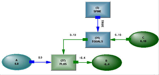The formula A = B + C, (partially represented in Figure 2) is a simple example of Constraint Reasoning. It forms a structure connecting the three variables A, B and C. Ranges of values can be ascribed to B and C, say 0 to 100 (0..100). Then the range of A is 0..200. Now, if any one of the variables is further constrained, the ranges on the other variables will immediately change. If A is constrained to have a range 0..50, then neither B nor C can have a value larger than 50. If B is further constrained to have a range 10..30, C cannot be larger than 40. The usefulness comes from the fact that the constraint is undirected in its operation - no decision was made as to what was being constrained by what, the connection of the elements through a structure made up of operators produced the constraint action. The structure can be extended in any direction, and influences can flow from any point to any other.

If the technique were only applicable to numbers, it would be useful but limited. The technique can be extended to handle logical constraints, as shown in Figure 3. The constraint is (poorly) represented in textual form by

IF A < B THEN C < D

The IF...THEN... operator in the text becomes an implication (IMP) operator, being controllable and having all the properties of first order logic - that is, it is invertible, it handles unknowable states, and it can exist in a quiescent state neither TRUE nor FALSE until at least one of its connections switches into a TRUE or FALSE state. The arrows represent the possible directions of information - if A is less than B, then information flows from that less than operator through the implication, or if C is greater than D, the information flow is the other way. If Control is not asserted, then FALSE can flow out of this pin. The constraint structure is again undirected, information flowing in whichever direction is relevant at the moment.

Logical constraints as well as purely numeric constraints can be controlled (using the equals in A=B+C), so the effects of decisions can alter the structure of the constraints. A controlling layer (the current highest level in the plan) can be turned into an undirected layer and a new controlling layer placed on top of it. The technique can be extended further to handle lists of objects and constraint structures which are dynamically created or modified within the plan in response to logical conditions.

The Constraint Reasoning Method (CRM) can be applied in the area of project management, where it can be made to look rather similar to CPM, in that there are activities, sequence constraints, resources. The undirected property of the base elements leads to much more flexible behaviour. The similarities between CPM and CRM will be described first, then the differences.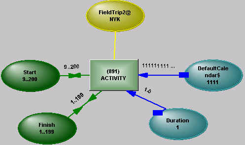

As illustrated in Figure 4 in slightly simplified form, a Constraint Reasoning activity has a Start Date node, a Finish Date node, a Duration node, and access to a calendar. The activity itself is represented by an active box in the network, which can calculate the Finish Date given the Start Date, Duration and calendar, or can calculate the Start Date given a Finish Date. The ACTIVITY box ensures that, at all times, the values at the Start Date, Duration, Finish Date and calendar connections are consistent with each other.

If the maximum number of days in the calendar is 1000, then to begin with, the Start Date and Finish Date nodes initially have a range of 1 to 1000.

This is not a consistent state for a duration of 10, because if the earliest Start Date is 1, then the earliest Finish Date is 10, and if the latest Finish Date is 1000, then the latest Start Date is 991. The ACTIVITY box makes the adjustments as soon as the ranges reach it, and then propagates the new values on its connections.

A CPM network is limited to one simple operation, the earliest start of a particular activity being the maximum of all its predecessors and everything in the plan must exist. The Constraint Reasoning network can have a wide range of logical and numerical analytic operators embedded in it and the existence of activities is controllable. All the constraints are initially not directed, the operators that make them up responding to the flow of information at their connections. There is no algorithm that understands planning, merely a messaging system mechanistically moving information through a network. The planner assembles the network using operators ranging from a low level "+" to add two numbers together, to an ACTIVITY operator representing the behaviour of an activity. In the ORION implementation of CRM, the large proportion of a typical plan that is low risk can be assembled as quickly as one would a CPM plan.

Complex Interaction At Operators

Resource constraint is an important aspect of CPM planning, but resource levelling is a relatively primitive operation because of its algorithmic basis. The Resource Usage operator in a CRM network typifies the non-algorithmic interaction among activities and resources that allows a much more realistic resource constrained analysis. The operator has several connections that carry ranges, and must respond to changes in those ranges, while being able to recover previous states.

A CRM Resource Usage operator is illustrated in Figure 7. It is normally connected to the start date for the activity, although it may be cascaded through durations of other usages, or any other logic needed to model particular effects. The Duration connection may be to the Activity duration, or some manipulation of it. There is a connection to a Resource, itself a list of operators maintaining bookings on a time basis. The Resource Intensity is the requirement for resource in each time period for a renewable resource. Ranges of values may be present on the Start day, Intensity, and Duration inputs. The Intensity and Duration connections may be linked together through an operator to give the effect of elasticity, a low resource intensity forcing a longer duration, and vice versa.

Either the Duration or Intensity ranges may include zero, allowing resource use to be turned off while maintaining existence of the activity. The Resource Intensity may include positive and negative values, the activity controlling the Usage potentially able to operate as a source or sink of resource.

The Start Hint is used to indicate where in the Start Date range the most preferred starting point would be, as early as possible to minimise project risk, as late as possible to minimise interest burden, late while preserving a safety zone, etc. The Hint controls the probability used when booking resources. Bookings do not occur until a TRUE flows in on Booking Control, allowing the response of a model without resource constraints to be investigated.

A hard booking by some other Usage may force the particular Usage to relinquish some of its tentative bookings, and it responds to this by cutting the range of its Start Date, and propagating the range out of the Start Date connection, limiting the starting range of the connected activity. If this Usage is to be hard booked, a singular value will come in on the Start Date connection. The Usage will undo tentative bookings outside the reduced range, and, if there is no zero in either the Duration or Intensity ranges, "bump" any other Usages which have tentative bookings affected by the hard booking. The Usage operator can also interact with Consumable Resources, with the lag between production and consumption made as complex as one desires.

The total bookings in each period on a resource are also accessible to be constrained. This is often a more useful metric than availability, as the plan can itself determine what is an appropriate availability for the resource after observing the usage.

The mechanism inside the Usage operator busily maintains consistency among the various ranges as the ranges fragment, and the availability of the resource fragments. This "busy agent" is doing the bidding of the user in a way not available to a resource levelling algorithm operating from outside the model, because here the algorithm is "inside", formed by the connections among the operators. This is what is meant by "non algorithmic" operation of the model.

The simplest use of Constraint Reasoning might be to tie the duration of one activity to the duration of another activity (Activity2 will take twice as long as Activity1), but the duration could instead be tied to the difference in starting times of two activities, or resource usage of another activity or any other identifiable or constructable point in the constraint network, whether or not project-related. That is, the method of analysis is general and extensible, as it must be to be adequately flexible.

The greater modelling freedom provided by CRM allows the inclusion of new types of activities and modelling in the project plan.

The CRM activity is logically controllable for existence - that is, it has a logical connection which turns it, and its effects, on and off. Straightforward activities, which must occur, are unconditionally set true. Activities with uncertainty can have logical interdependencies which enable them to compete with other activities for existence. The logical control can come from any other point in the model, or can flow from this activity to any other point.

Sometimes there is sufficient uncertainty to justify the building in of mutually exclusive alternatives, one of which will be decided upon depending on what else occurs (something as simple as choosing between building a hotel or a marina, or perhaps different technologies to produce similar outcomes). One path might be shorter but more expensive, or involve development and have higher risk, but have longer in-service life. The logic deciding between the two paths is built into the network, and can draw on as many influences as desired. The two alternative paths can themselves be mini-projects, and don't need to have common starting and ending points as shown in the diagram. If there is no analytic basis for choosing between the two paths, then probabilistic control can be asserted on which path is chosen. If desired, random number generators can be embedded in the plan (and control asserted over them, and so on).

Some activities in a plan may have risks associated with them - risks that they may not occur, or that their duration will become extended. There are two ways of handling this, namely using backup activities and contingent activities.

A Backup activity is worked on in parallel with the activity having duration risk. The backup activity may take longer to complete than the minimum duration for the main activity. However, if the duration of the main activity does become extended, the work spent on the backup activity has been good insurance for getting the project finished near the initial deadline.

Contingent activities can be embedded in the plan, ready to be scheduled if failure occurs on some primary activity. As distinct from backup activities, work on the contingent activity only begins when failure has occurred on the primary activity. If the primary activity succeeds, the duration of the contingent activity is forced to zero, rendering the activity nonexistent.

The point of building the contingent activity into the risk model is that it is made clear to others how risks are being minimised. If the duration of the project is strongly constrained so that the contingent activity is forced out of existence (there is no slack to accommodate its minimum duration), the risk of the project can be made to increase, reflecting the fact there is now no contingency against failure.

Normally an activity will have TRUE asserted on its Control pin, meaning that it unconditionally exists and should maintain consistency on all its connections. If the existence of an activity is not yet fixed, it observes changes taking place on its Start and Finish connections. If the maximum possible duration between the Start and Finish values becomes less than its minimum real duration, the ACTIVITY switches its duration to zero and sends FALSE out of its Logical Control pin. The Activity cannot be TRUE, because to be so would require it to accept inconsistent states on its connections. When the Control pin is FALSE, any connection between Start and Finish is lost, preventing precedence constraints from being effective through the non-existent activity. If the Control pin is connected through an exclusive OR to another activity, the other ACTIVITY will be forced to exist.

A constraint on cost can feed back through the logic in the plan to force the duration to zero, or a lack of resources may similarly force the activity out of existence.

CRM easily models this logical switching among alternatives in the plan activated by conditions within the plan. Attempting to use external risk analysis on a CPM network for this complex behaviour is difficult to the point of futility as the plan changes its topology.

Other ways of handling risk are available. As the plan is developed, a cost versus risk profile of the project should have become apparent, pointing to ways in which the risk can be reduced without increasing cost.

A simple way to push high risk activities towards the start of the project is to make the activities book a particular risk as a resource, and make the cost of the resource rise with time. A minimum cost schedule will cluster the high risk activities at the start of the project. Some high risk activities may need to be delayed for other reasons, but then additional modelling can be used to protect against their failure.

With CPM and similar directed planning tools, a cashflow can be experimented with while activities are fixed in time, or activities can be moved about with primitive cashflow output. Constraint Reasoning allows the user to constrain activities and observe cashflow, or constrain cashflow and observe the effect on activities as the cashflow constraint pushes them around. Other planning constraints such as NPV may be added to the plan, coming into effect as the variability in activity placement reduces.

NPV is a simple way of determining the relative worth of a project by reducing the cashflow to a single number. For an investment in a project, NPV is calculated on a cashflow which will typically look like Figure 14, where all the variability has been stripped from the project by making firm assumptions about where everything will occur, and the cashflow in each period.

It is more useful to allow some variability to remain in the scenario, to get bounds on the possible NPV to aid in making other related decisions. Cashflow is one example where bookings of a resource are being constrained. The cashflow diagram shows variability of magnitude and risk of slipping. Without these being present, the person who interprets the NPV must look to other measures to assess the project risk.

With a range for the NPV, it is then simple to make this a directly user controllable constraint, so the user in effect has a knob to turn and may observe the results interactively, or may connect it analytically to some other point in the plan, possibly a corporate goal, and have this feed back into the decision-making process. The structure used to evaluate NPV is undirected so changes to amounts per period or interest rates can ripple in either direction through the constraint structure.

With other metrics also acting as constraints (risk versus time, maximum exposure) and interacting with each other, the people developing the project plan are "directed" along the corporate path, and are much less likely to produce a good NPV figure for the project based on invalid assumptions, assumptions that had to be made when there was no way of carrying variability forward in the analysis. As shown in Figure 16, other stakeholders are able to exert constraints directly on the plan while its structure is variable. The planners must now find a path through or around these constraints, and in doing so, they have minimised the risks expressed through the constraints.

With components that allow variability in the project plan, the area being analysed can be extended. Some projects, typified by high rise buildings, can be viewed in a very sequential way with little regard for other factors. Once the decision has been made on what to build, the project moves through the stages of design (How), tendering (How Much) and construction (How Long). Only rarely do previous decisions have to be revisited.

Development projects, on the other hand, tend to be a swirl of interactions among the What, the How, the How Long and the How Much. CRM can be used starting with the Mission Statement - the What of the project. Ranges and logical alternatives permit description of the potential variability of outcome during the Requirements Elicitation stage.

The initial model may have no sense of time, just being the constraints that operate on the expected outcome. The model is operating at the level of Strategic Planning, supporting (or invalidating) the initial implementation decision. If this process is followed, the project plan will automatically include project termination criteria - the model was used to determine whether to go ahead, so it already has an analysis of the project's worth to the organisation. Further modelling can then be introduced to firm up options and flesh out details - what alternative approaches or technologies might be used. The next stage may be to analyse tenders which do not exactly match the requirements. A further stage sees the model expanded into a detailed implementation plan, where the What, Why, How, How Long and How Much are connected through a web of constraints which has grown naturally as the plan developed. Altering any of the constraints can potentially affect any or all of the aspects of the project, including its existence.

Conclusion

This paper has presented a brief overview of Constraint Reasoning when used to model projects involving uncertainty. The technique is a general method of analysis which is not predicated on a rigid and preconceived notion of how planning should work, as are CPM and spreadsheets.

The Constraint Reasoning model allows the introduction and evaluation of many aspects that would be very difficult to handle in a conventional risk analysis of a rigid (and brittle) project plan. The flexibility of Constraint Reasoning eliminates the artificial distinction between planning and risk analysis. It is just as applicable in Program Management and Strategic Planning as it is in Project Planning, allowing a single planning tool to support decision making throughout the life cycle of the project.

The Constraint Reasoning elements described in this paper are implemented in the ORION analytic system, allowing users to develop planning models in areas poorly served by the current methods of analysis.

Linking Statistical Risks

Home