Constraint Reasoning

Constraint reasoning has a very simple basis. Say we have an equation

    X + Y = 10

and we know that X and Y are somewhere in the range 0..10 (we will assume integer ranges for now).

In this case, X could be 10 and Y would be 0, or vice versa, so the equation does not constrain the values of X and Y.

If we have the equation

    X - Y = 4

then X cannot be less than 4, and Y cannot be more than 6.

If we combine the two equations, but examine each individually, we are no further ahead. However, if we cut one of the ranges in half, and examine both halves, we find that, for X in 4..7, Y would be 3..6 using one equation, and 0..3 in the other, with the only common value of 3. Using the other half of the range for X of 8..10, we find ranges for Y of 0..2 and 4..6, with no common value. We conclude that the value of Y is 3 and the value of X is 7.

Splitting the ranges in half and examining the effect is an example of hypothesising - we tried something and observed the result. We then needed to put back the values the way they were, to try something else - this is backtracking. We can backtrack on values, and we can also backtrack on any changes we may have made to the structure - we might have added a variable or an operator, made new connections or destroyed some structure - we can backtrack on any of these changes because we store an image of the particular part of the structure before we change it.

We can easily extend the method to inequations like

    X + Y <= 10

or more complicated equations, like

    Stress = W*L^3/48*E*I

(we will need real numbers, but that is easily done).

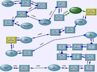
When we have more complicated equations, we need to perform the constraint reasoning at the individual operators, rather than just at the variables (we always do it at the operators). If we look internally at the equation, we find a structure that looks like

so we might find ourselves at a PLUS operator or an EXP or LN. We perform the constraint reasoning analysis at the operator, then move the new values to the operator at the other end of the connection where the range changed, and so on until there is nothing left to change.

We have used numbers to demonstrate the principle, but we can prune sets of objects just as well as ranges of numbers.

The principle of Constraint Reasoning is that the answer lies in the posing of the question - we start with ranges that encompass the answer, and by reducing those ranges in accordance with the constraints, we will end with a result which is in accordance with all the constraints. That doesn't mean we will come up with single values - if all we had was the relation X + Y = 10, then the initial ranges on X and Y would not have changed at all.

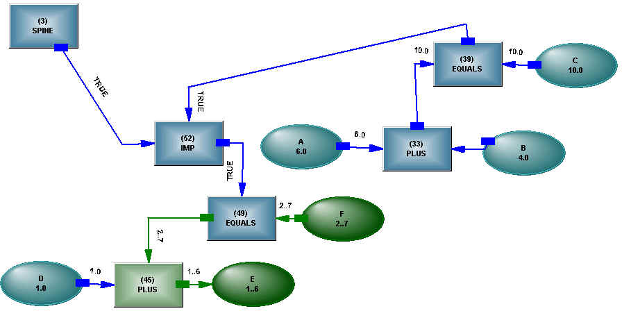
We can couple logic into the process - here is an implication structure.

IF A + B = C THEN D + E = F

There are six numeric variables here - A, B, C, D, E, F. Let's say we only initially know ranges of 0..10. As the ranges shrink, we may find that A + B = C, which causes a true to flow out of one EQUALS, through the implication, and cause another constraint to be added to D, E, F - that is, D + E = F. Or, instead, we may find that D + E <> F, which causes a false to flow out of the EQUALS, back through the implication, and result in the constraint A + B <> C. It is also possible that we don't know whether the implication is true or not, and we find A + B = C and D + E <>F, which would cause a False to flow out of the implication. By performing constraint reasoning at the operator, we can use structures in many ways.

Extensions to Constraint Reasoning

Inheritance Pruning

The normal method of pruning assumes direct direct comparison of ranges, but with objects, sometimes it is necessary to take inheritance into account - a present participle is consistent with a participle. See ANDPARSE for an operator which uses inheritance during pruning.

Localised Alternatives

The basic principle of Constraint Reasoning is that all the possibilities exist at the start of the reasoning. Sometimes this is not a good idea - you do not hand out grenades to soldiers who are not on active duty, because they might blow themselves up. The same principle can apply in a model - alternatives only become available under certain conditions - see ADDPROPERTY.

Hotwired Constraints

It is possible for a user to add constraints during the Constraint Reasoning process - see Constraint Reasoning in Project Management. This is possible because the reasoning is not stuck up its stack, but is occurring in a grounded structure.

Interwoven Structure Building

Constraint Reasoning can seem very fussy, with its need for the posing of the problem to encompass the solution. Such a limitation does not lend itself to dynamic construction of a Constraint Reasoning problem. With the ability to weave structure building into CR, the fussiness has gone. The two techniques can work together synergistically, to build a structure that encompasses the solution,  guided by CR. Active Maps exemplify this approach.

See:

Backtracking

Constraint Reasoning in Parsing

Constraint Reasoning in Prepositional Maps

Constraint Reasoning in Diffuse Operators

Home